Difference between revisions of "MGED CMD simulate"
| Line 103: | Line 103: | ||
|} | |} | ||
<br style="clear: both" /> | <br style="clear: both" /> | ||
| − | In order to see what we did so far we should set the view for the geometry we have so far. We will use an "ae 35 15", that means the | + | In order to see what we did so far we should set the view for the geometry we have so far. We will use an "ae 35 15", that means the azimuth angle is at 35 degrees and the elevation at 15 degrees.The angle of elevation of an object as seen by an observer is the angle between the horizontal and the line from the object to the observer's eye (the line of sight).The azimuth of an object is the angular distance along the horizon to the location of the object.We will use autoview" command to reset the view size and the view center such that all displayed objects are within the view. And then we will do a translation on the Y axis. |
<br> | <br> | ||
{|align="left" | {|align="left" | ||
| Line 228: | Line 228: | ||
|} | |} | ||
<br style="clear: both" /> | <br style="clear: both" /> | ||
| − | In order to create an animation from your simulation, you will have to run the script below. It simulates the cube falling on the ground every step for 190 steps(after the 190th step the simulation stops rendering images, it discovers it had collided with the ground plane) and then it renders an image(for every step) with the specified elevation view (in degrees is being specified). The "rt" command executes the BRL-CAD rt program with the default options. The default dimensions for the image are 512x512pixels, that can be changed and it is changed for the purpose of this tutorial providing the -w(width) and -n(height) options. The -a option gives us the | + | In order to create an animation from your simulation, you will have to run the script below. It simulates the cube falling on the ground every step for 190 steps(after the 190th step the simulation stops rendering images, it discovers it had collided with the ground plane) and then it renders an image(for every step) with the specified elevation view (in degrees is being specified). The "rt" command executes the BRL-CAD rt program with the default options. The default dimensions for the image are 512x512pixels, that can be changed and it is changed for the purpose of this tutorial providing the -w(width) and -n(height) options. The -a option gives us the azimuth angle(The azimuth of an object is the angular distance along the horizon to the location of the object.), like before. The -e option provides the elevation angle(The angle of elevation of an object as seen by an observer is the angle between the horizontal and the line from the object to the observer's eye (the line of sight). The current database name is added to the end of the rt command line along with either the specified objects or, if none is specified, the list of currently displayed objects. We will add the 2 objects that we actually want the simulation for, sim_gp.r and sim_cube.r . |
<br> | <br> | ||
{|align="left" | {|align="left" | ||
| Line 246: | Line 246: | ||
<br style="clear: both" /> | <br style="clear: both" /> | ||
| + | Now that we have a bunch of pictures we want to actually see the cube falling to the ground, we could watch the pictures on a slide-show, but we can do better than that. We will make a *gif and a *mpg movie out of our pictures. For that you need to install the latest ImageMagick software on Linux , just type : | ||
| + | <br> | ||
| + | {|align="left" | ||
| + | |<pre> | ||
| + | brlcad@brlcad: sudo apt-get install imagemagick | ||
| + | </pre> | ||
| + | |} | ||
| + | <br style="clear: both" /> | ||
| + | {|align="right" | ||
| + | |[[Image:Simulation_large.gif|thumb|256px|Cube falling to the ground plane gif without the viewset, modeled and rendered in BRL-CAD]] | ||
| + | |} | ||
| − | + | You will get some dependencies that you must install before installing the ImageMagick package, install those. After everything has been installed, move to the folder where you have your images saved and run the following command: | |
| + | <br> | ||
| + | {|align="left" | ||
| + | |<pre> | ||
| + | brlcad@brlcad: convert *png simulation.gif | ||
| + | brlcad@brlcad: convert *png simulation.mpg | ||
| + | </pre> | ||
| + | |} | ||
| + | <br style="clear: both" /> | ||
| + | That is it, now you can watch a gif/movie of your simulation. | ||
| + | |||
| + | Well, that's great, but lets stop the view from constantly changing and make it look better for that we will use the ae3515.rt file we saved awhile back in our tutorial. Back then we set the view for the whole scene, giving an azimuth angle(the -a option) and an elevation angle(the -e option). We translated the position of our geometry with 10 units on the Y axis and we also used "autoview" command, to capture in the window size the whole geometry. | ||
| − | To add the saved view from the saved file to your own rt script, you have to open the az3515.rt saved file with a text editor program, say gedit on Linux systems, and copy paste the info from starting with the "$*\" and ending with the second "EOF" line. What do those lines do? They specify the location of your database and the top regions from it that you want to take place in the simulation, much likely the "rt [- options] sim.g | + | To add the saved view from the saved file to your own rt script, you have to open the az3515.rt saved file with a text editor program, say gedit on Linux systems, and copy paste the info from starting with the "$*\" and ending with the second "EOF" line. What do those lines do? They specify the location of your database and the top regions from it that you want to take place in the simulation, much likely the "rt [- options] sim.g sim_gp.r sim_cube.r" command, only now you give the whole path to your sim.g file and in there you use the sim_gp.r and sim_cube.r regions. Now lets explain those numbers that we just copy-pasted : |
* viewsize is a variable to resize the screen through software; | * viewsize is a variable to resize the screen through software; | ||
* orientation is placement of an object in a rotational coordinate system (XYZ in our case) with respect to a fixed point and a reference position; | * orientation is placement of an object in a rotational coordinate system (XYZ in our case) with respect to a fixed point and a reference position; | ||
* eye_pt is the point at which the eye is placed when looking at the scene. | * eye_pt is the point at which the eye is placed when looking at the scene. | ||
| − | The -M option for the rt command specifies that you are going to provide a view script for a file, that's what you are doing between the 2 EOF lines. | + | The -M option for the rt command specifies that you are going to provide a view script for a file, that's what you are doing between the 2 EOF lines. Then we give the width and height we want our image to be. You can try and modify it, to get different size images. The rtedge command will render a hidden-line image of the specified geometry database model and uses the same script we provided for the rt command, with the -M option. The -c option specifies auxiliary commands, in our case we set the override to 1. |
| − | |||
<br> | <br> | ||
{|align="left" | {|align="left" | ||
| Line 261: | Line 282: | ||
# simulate.sh | # simulate.sh | ||
######################################################################## | ######################################################################## | ||
| − | |||
for i in `seq 1 190` ; do | for i in `seq 1 190` ; do | ||
echo "Simulating..." | echo "Simulating..." | ||
| − | mged sim.g simulate $i | + | bin/mged sim.g simulate $i |
echo "Raytracing..." | echo "Raytracing..." | ||
rt -M -w 360 -n 640 -W -F5 \ | rt -M -w 360 -n 640 -W -F5 \ | ||
$*\ | $*\ | ||
'/home/brlcad/brlcad/sim.g'\ | '/home/brlcad/brlcad/sim.g'\ | ||
| − | ' | + | 'sim_gp.r' 'sim_cube.r'\ |
2>> sim.log\ | 2>> sim.log\ | ||
<<EOF | <<EOF | ||
| Line 278: | Line 298: | ||
start 0; clean; | start 0; clean; | ||
end; | end; | ||
| − | + | EOF | |
| − | + | rtedge -M -w 360 -n 640 -W -F5 -c "set ov=1"\ | |
| − | |||
$*\ | $*\ | ||
'/home/brlcad/brlcad/sim.g'\ | '/home/brlcad/brlcad/sim.g'\ | ||
| − | ' | + | 'sim_gp.r' 'sim_cube.r'\ |
2>> sim.log\ | 2>> sim.log\ | ||
<<EOF | <<EOF | ||
| Line 291: | Line 310: | ||
start 0; clean; | start 0; clean; | ||
end; | end; | ||
| − | + | EOF | |
| − | |||
echo "Generating image..." | echo "Generating image..." | ||
run fb-png -F5 -w 360 -n 640 image$i.png | run fb-png -F5 -w 360 -n 640 image$i.png | ||
| − | |||
echo "image"$i".png done" | echo "image"$i".png done" | ||
done | done | ||
| − | kill % | + | kill %i |
| − | |||
| − | |||
| − | |||
| − | |||
| − | |||
| − | |||
| − | |||
| − | |||
</pre> | </pre> | ||
|} | |} | ||
<br style="clear: both" /> | <br style="clear: both" /> | ||
| + | |||
{|align="right" | {|align="right" | ||
|[[Image:Simulation_256x256.gif|thumb|256px|Cube falling to the ground plane gif with the viewset, modeled and rendered in BRL-CAD]] | |[[Image:Simulation_256x256.gif|thumb|256px|Cube falling to the ground plane gif with the viewset, modeled and rendered in BRL-CAD]] | ||
|} | |} | ||
| − | |||
| − | |||
| − | |||
| − | |||
| − | |||
| − | |||
| − | |||
| − | |||
| − | |||
| − | |||
| − | |||
| − | |||
| − | |||
| − | |||
| − | |||
For the movies, here are youtube links : | For the movies, here are youtube links : | ||
Revision as of 16:51, 14 September 2012
BRL-CAD recently integrated a new command in its mged tool, the simulate command. To simulate a cube falling to the ground plane one should follow those steps in order to run it in the mged tool.
BRL-CAD is a CSG (Constructive Solid Geometry) program. The representation is done in a system of axis XYZ. The XY axis is the ground axis, so you should make sure later in the tutorial that your ground plane (referenced as "gp") is being parallel with this axis.
First open the mged tool, if you have BRL-CAD installed on your Linux system it should be easy, just type mged in a terminal and a mged terminal should open.
brlcad@brlcad: mged |
In the mged terminal select the File menu, and then the New... (file dialog button). A window will appear and a name for your new database will be required. For the purpose of this tutorial we will name the new database, sim1. Introduce the chosen name (sim1) in the "File name:" field and hit save.
Now you have opened a new database. Next we want to add some geometry to the database. Something that we will have to simulate on.
In the mged command window we will now type the following series of commands :
mged> in Enter name of solid: cube Enter solid type: rpp Enter XMIN, XMAX, YMIN, YMAX, ZMIN, ZMAX: -1 1 -1 1 -1 1 |
The "in" command creates new geometry, it allows the user to type in the arguments to create a shape with the name provided by the second argument, in the example above is the name provided when "Enter name of solid:" appears on the screen. The arguments of the in command can be provided one by one, as in the example above or in one single line, like in the example below:
mged> in cube rpp -1 1 -1 1 -1 1 |
We have so far a box, now we want to add a ground plane to our simulation. Now is the moment to remember that the XY axis is the ground axis, so out plane should be parallel to it, that's why we first introduce the lengths of the the ground plane and then we introduce the "thickness", in our case 2mu. The Z axis is up, so the -1mu and +1mu on it gives the "thickness" of our ground plane. The ground plane must be name "gp", that's the way the program knows that you are defining a surface that will play the role of the ground. After creating regions, the ground region will be named "gp.r" so that the simulation will know that it is actually the plane on which you want your objects to fall onto.
(*mu = measuring units, by default it is mm)
mged> in gp rpp -15 15 -15 15 -1 1 |
You should see now 2 boxes on your screen, one perpendicular on the other one, with a little overlap between them.
Using the sed command we will select the box and translate it 100 units on the Y axis.
mged> sed cube mged> tra 0 0 50 mged> accept |
To be able to run the simulate command our geometry shapes should be grouped in regions to do this we will use the "r" command and create 2 regions for the box and the ground shapes.
mged> r cube.r u cube mged> r gp.r u gp |
We want our ground plane and cube to have color and material properties, for a nicer visual aspect. We add material properties to regions in BRL-CAD with the "mater" command, just type "mater cube.r" in the mged window, you will get a step by step tutorial.
After hitting enter you will be asked specify the shader type, type "plastic {tr 0.2 re 0.2}" without the quotes, the tr(transparency) is set to 20% same with the reflexivity. Then we want to choose a color for our texture, the color is a combination of the 3 RGB basic colors(Red/Green/Blue) - the colors intensity varies between 0-255, 0 for a color means that that color will not appear in the combination,255 means that color is at its most intense, we will choose for the cube a strong red so we type "255 0 0". When we are asked if we want the shader's object to override the lower nodes we choose yes, we want the object to look uniform.
mged> mater cube.r
Current shader string =
Specify shader.  Enclose spaces within quotes.  E.g., "light invisible=1"
Shader? ('del' to delete, '.' to skip) "plastic {tr 0.2 re 0.2}"
Current color = (No color specified)
R, G, B color values (0 to 255)? ('del' to delete, '.' to skip) 255 0 0
Current inheritance = 0: lower nodes (towards leaves) override
Should this object's shader override lower nodes? ([y/n] or '.' to skip) y
|
We can specify all those parameters in one single line :
mged> mater cube.r "plastic {tr 0.2 re 0.2}" 255 0 0 y
|
We do the same for the ground plane region, but we set the color to blue :
mged> mater gp.r "plastic {tr 0.2 re 0.2}" 0 0 255 y
|
In order to see what we did so far we should set the view for the geometry we have so far. We will use an "ae 35 15", that means the azimuth angle is at 35 degrees and the elevation at 15 degrees.The angle of elevation of an object as seen by an observer is the angle between the horizontal and the line from the object to the observer's eye (the line of sight).The azimuth of an object is the angular distance along the horizon to the location of the object.We will use autoview" command to reset the view size and the view center such that all displayed objects are within the view. And then we will do a translation on the Y axis.
mged> ae 35 15 mged> autoview mged> tra 0 10 0 |
We want to save this view for later so we will run the saveview command :
mged> saveview ae3515.rt |
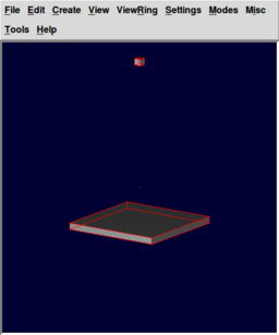
Before we run the simulation command let's see what does our geometry look like so far:
mged> rt -W |
You should get an image similar to the one to the right :
Now we are ready to run the simulate command:
mged> simulate 100 |
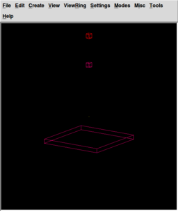
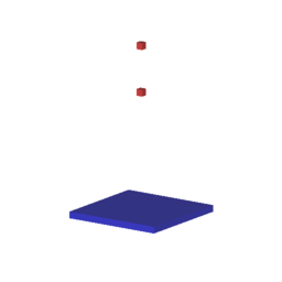
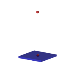
After the simulation runs its course you should see the 2 cubes and the ground plane like in the image to the right. Actually there are not 2 cube, there is just one cube with 2 positions, the previous position (red) and the current position(pink). The ground plane has only the current position(which is the same with the previous position, the ground does not move). We will use the "who" command to find out what objects are being displayed.
mged> who |
You should get the following answer:
cube gp sim.c |
Now, we don't really want to display the box and the ground shapes, we already have them in the "sim.c" group so we will unload all the geometry(using the "Z" command).
mged> Z |
Though it might look like the "sim.c" group contains exactly what we need for our simulation, that it is not necessarily true. So lets see what "sim.c" contains using the "l" command(The "l" command displays a verbose description about the specified list of objects.):
mged> l sim.c
 Ged_list from the libged library [-r] [-t] <objects>
 sim.c:  --
    u sim_gp.r
    u sim_cube.r
    u bb_reg_sim_gp.r
    u bb_reg_sim_cube.r
|
So as we can see the "sim.c" group does not contain only the geometry we want to use in our simulation. Actually at first sight it does not look to contain the desired geometry at all. Well the sim_gp.r and sim_cube.r is what we are looking for, the simulate command renames the geometry it uses for simulation, adding the prefix "sim_" in front of every one of them. The other 2 regions we see here (bb_reg_sim_gp.r and bb_reg_sim_cube.r) are the bounding-boxes regions of the geometry and they are used by the bullet engine. So we only need the 2 "sim_" prefixed regions. We will display them using the "draw" command.
mged> draw sim_gp.r mged> draw sim_cube.r |
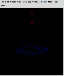
To see the difference the simulation made we will also display the cube.r region, and use "autoview" to fit all the geometry in the window, you should see something like the image to the right :
mged> draw cube.r mged> autoview mged> tra 0 10 0 |
You should get an image similar to the one to the right :
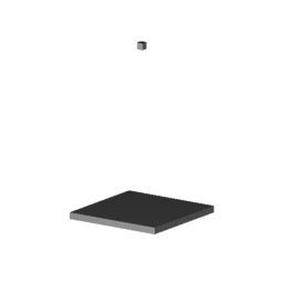
Now to actually see the simulation we will raytrace it, using the "rt" command.
mged> rt -W |
The raytraced image should look like this one :
If you want to see when the cube touches the ground plane then you only have to increase the simulate step numbers to 190. You should see something like the image to the right :
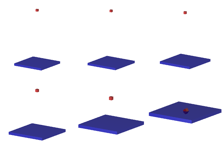
In order to create an animation from your simulation, you will have to run the script below. It simulates the cube falling on the ground every step for 190 steps(after the 190th step the simulation stops rendering images, it discovers it had collided with the ground plane) and then it renders an image(for every step) with the specified elevation view (in degrees is being specified). The "rt" command executes the BRL-CAD rt program with the default options. The default dimensions for the image are 512x512pixels, that can be changed and it is changed for the purpose of this tutorial providing the -w(width) and -n(height) options. The -a option gives us the azimuth angle(The azimuth of an object is the angular distance along the horizon to the location of the object.), like before. The -e option provides the elevation angle(The angle of elevation of an object as seen by an observer is the angle between the horizontal and the line from the object to the observer's eye (the line of sight). The current database name is added to the end of the rt command line along with either the specified objects or, if none is specified, the list of currently displayed objects. We will add the 2 objects that we actually want the simulation for, sim_gp.r and sim_cube.r .
#!/bin/sh
#				simulate.sh
########################################################################

for i in `seq 1 190` ; do
		echo "Simulating..."
		mged sim.g simulate $i
		echo "Raytracing..."
                rt -a 35 -e 15 -o image$i.png sim.g sim_gp.r sim_cube.r
done
|
Now that we have a bunch of pictures we want to actually see the cube falling to the ground, we could watch the pictures on a slide-show, but we can do better than that. We will make a *gif and a *mpg movie out of our pictures. For that you need to install the latest ImageMagick software on Linux , just type :
brlcad@brlcad: sudo apt-get install imagemagick |
You will get some dependencies that you must install before installing the ImageMagick package, install those. After everything has been installed, move to the folder where you have your images saved and run the following command:
brlcad@brlcad: convert *png simulation.gif brlcad@brlcad: convert *png simulation.mpg |
That is it, now you can watch a gif/movie of your simulation.
Well, that's great, but lets stop the view from constantly changing and make it look better for that we will use the ae3515.rt file we saved awhile back in our tutorial. Back then we set the view for the whole scene, giving an azimuth angle(the -a option) and an elevation angle(the -e option). We translated the position of our geometry with 10 units on the Y axis and we also used "autoview" command, to capture in the window size the whole geometry.
To add the saved view from the saved file to your own rt script, you have to open the az3515.rt saved file with a text editor program, say gedit on Linux systems, and copy paste the info from starting with the "$*\" and ending with the second "EOF" line. What do those lines do? They specify the location of your database and the top regions from it that you want to take place in the simulation, much likely the "rt [- options] sim.g sim_gp.r sim_cube.r" command, only now you give the whole path to your sim.g file and in there you use the sim_gp.r and sim_cube.r regions. Now lets explain those numbers that we just copy-pasted :
- viewsize is a variable to resize the screen through software;
- orientation is placement of an object in a rotational coordinate system (XYZ in our case) with respect to a fixed point and a reference position;
- eye_pt is the point at which the eye is placed when looking at the scene.
The -M option for the rt command specifies that you are going to provide a view script for a file, that's what you are doing between the 2 EOF lines. Then we give the width and height we want our image to be. You can try and modify it, to get different size images. The rtedge command will render a hidden-line image of the specified geometry database model and uses the same script we provided for the rt command, with the -M option. The -c option specifies auxiliary commands, in our case we set the override to 1.
#!/bin/sh
#				simulate.sh
########################################################################

for i in `seq 1 190` ; do
	echo "Simulating..."
	bin/mged sim.g simulate $i
	echo "Raytracing..."
	rt -M -w 360 -n 640 -W -F5 \
        $*\
        '/home/brlcad/brlcad/sim.g'\
        'sim_gp.r' 'sim_cube.r'\
        2>> sim.log\
        <<EOF
        viewsize 5.85714285714286e+01;
        orientation 2.81094745635754e-01 5.39977982351790e-01 7.03713007376454e-01 3.66329804684860e-01;
        eye_pt 9.91586132512701e+01 6.94316084769606e+01 5.37880960360133e+01;
        start 0; clean;
        end;
EOF
	rtedge -M -w 360 -n 640 -W -F5 -c "set ov=1"\
        $*\
        '/home/brlcad/brlcad/sim.g'\
        'sim_gp.r' 'sim_cube.r'\
        2>> sim.log\
        <<EOF
        viewsize 5.85714285714286e+01;
        orientation 2.81094745635754e-01 5.39977982351790e-01 7.03713007376454e-01 3.66329804684860e-01;
        eye_pt 9.91586132512701e+01 6.94316084769606e+01 5.37880960360133e+01;
        start 0; clean;
        end;
EOF
	echo "Generating image..."
	run fb-png -F5 -w 360 -n 640 image$i.png
	echo "image"$i".png done"
done
kill %i
|
File:Simulation 256x256.gif Cube falling to the ground plane gif with the viewset, modeled and rendered in BRL-CAD |
For the movies, here are youtube links :
- movie out of the simulation with the viewset : http://youtu.be/XS1wUnQ8q0M
- movie out of the simulation without the viewset : http://youtu.be/f-04dvJ7iIQ
(* the install commands are for the Ubuntu - distributions, you must use your package manager for installing ImageMagick on your own Operating System)
