Difference between revisions of "DSP"
(→Creating a DSP object from manual or programmatic generation of data) |
(→Importing DSP data into a .g file) |
||
| Line 81: | Line 81: | ||
In mged create a dsp object: | In mged create a dsp object: | ||
| − | mged> in | + | mged> in dsp1.s dsp f Ex1.dsp 142 150 0 ad 1 0.005 |
| + | mged> r dsp1.r u dsp1.s | ||
Example 2. | Example 2. | ||
| Line 88: | Line 89: | ||
mged> in dsp2.s dsp f Ex2.dsp 152 150 0 ad 1 0.005 | mged> in dsp2.s dsp f Ex2.dsp 152 150 0 ad 1 0.005 | ||
| − | + | mged> r dsp2.r u dsp2.s | |
| − | |||
=== Rendering your DSP === | === Rendering your DSP === | ||
Revision as of 06:15, 11 June 2012
Contents
Displacement (DSP) map primitive
Creating a DSP object from miscellaneous images
We will use two examples to illustrate the next few sections.
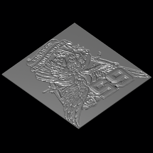
1. A black and white (gray scale) image (png format):
with properties:
$ file Ex1.png
Ex1.png: PNG image, 142 x 150, 8-bit gray+alpha, non-interlaced
2. A color png file:
with properties:
$ file Ex2.png
Ex2.png: PNG image, 152 x 150, 8-bit/color RGBA, non-interlaced
Preparing your height field data
The DSP takes unsigned short (16-bit) integer data. Our various command-line data converters can help bring data in from pretty much any existing format, including image data, via various processing commands. If the data was in png image format, for example (which is basically 3-channel 8-bit integer data), the data could be prepared with a combination of 'png-pix', 'pix-bw', and 'cv'.
If you type the 'in' command, it will prompt you for each parameter individually and that should help some. For the DSP, the main parameters are: the source of the height data, the width (number of points in the Y direction) and length (number of points in the X direction) of the input data, width/length/height scaling factors, and whether to smoothly interpolate between cells (0 = do not interpolate, 1 = interpolate).
See the 'dsp_add' tool for combining two existing DSP data files into one.
A DSP primitive is an array of cells initially defined by points in the XY plane as positive heights from Z = 0. The DSP can then be transformed to other orientations and positions. The number of cells is (numX * numY).
The data format for the DSP primitive is network-ordered unsigned short integers (nu16). BRL-CAD has a couple of dozen tools that you can use for converting existing data into that raw format, such as the 'cv' command or the 'bw-d' and 'd-u' commands among other similar tool chains. If you use the cv command, the output format is "nus" for network unsigned shorts.
Using the two examples to convert the data to dsp format.
Example 1.
Convert it to a bw file (one pixel is one unsigned char):
$ png-bw Ex1.png > Ex1.bw
View the result:
$ bw-fb -w142 -n150 Ex1.bw
Convert it to the format required for a dsp file (nu16):
$ cv huc nu16 Ex1.bw Ex1.dsp
Example 2.
Convert it to a pix file (one pixel is defined by three unsigned chars):
$ png-pix Ex2.png > Ex2.pix
View the result:
$ pix-fb -w152 -n150 Ex2.pix
Convert it to a bw file (one pixel is one unsigned char):
$ pix-bw Ex2.pix > Ex2.bw
View the result:
$ bw-fb -w152 -n150 Ex2.bw
Convert it to the format required for a dsp file:
$ cv huc nu16 Ex2.bw Ex2.dsp
Importing DSP data into a .g file
Example 1.
In mged create a dsp object:
mged> in dsp1.s dsp f Ex1.dsp 142 150 0 ad 1 0.005
mged> r dsp1.r u dsp1.s
Example 2.
In mged create a dsp object:
mged> in dsp2.s dsp f Ex2.dsp 152 150 0 ad 1 0.005
mged> r dsp2.r u dsp2.s
Rendering your DSP
Example 1.
mged> B dsp.s
mged> ae 45 45
mged> rt
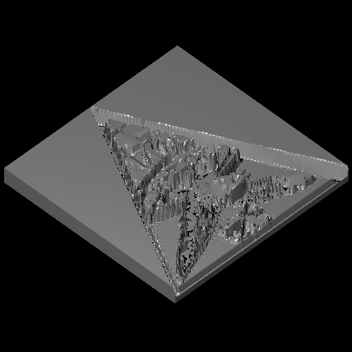
You should see something like this:
You can play around with the scaling factors (the end pair: 1 - cell width, 0.005 - cell height) to improve the looks of the image.
But now let's invert the file so we get its negative:
$ bwmod -m-1 -a255 < Ex1.bw > Ex1neg.bw
And make another dsp:
Example 2.
mged> B dsp2.s
mged> ae 45 45
mged> rt
You should see something like this:
Again, you could play with various parameters to get the desired look.
Creating a DSP object from manual or programmatic generation of data
Now let's consider a more practical example and a real test of BRL-CAD. We can import topological data and produce a realistic ground surface. There are many free sources of such data. See this site for a start:
http://www.naturalgfx.com/free_topo_gis.htm
We started with shapefile data for the US from:
http://seamless.usgs.gov/data_availability.php?serviceid=Dataset_19
We downloaded the zip archive 'ned_19_arc.zip' and unzipped in its own directory:
$ mkdir ned_19_usa_arcgis_shapefile
$ mv ned_19_arc.zip ned_19_usa_arcgis_shapefile
$ cd ned_19_usa_arcgis_shapefile
$ unzip ned_19_arc.zip
Archive:  ned_19_arc.zip
  inflating: ned_19_arc.dbf
  inflating: ned_19_arc.pdf
  inflating: ned_19_arc.prj
  inflating: ned_19_arc.sbn
  inflating: ned_19_arc.sbx
  inflating: ned_19_arc.shp
  inflating: ned_19_arc.shp.xml
  inflating: ned_19_arc.shx
  inflating: ned_19_arc.txt
  inflating: ned_19_arc.xml
  inflating: NED_DataDictionary2006.pdf
See these pages for details of the [ESRI] shapefile format:
http://www.esri.com/library/whitepapers/pdfs/shapefile.pdf
http://en.wikipedia.org/wiki/Shapefile
We will use one of two Perl modules, Geo::Shapelib or Geo::ShapeFile, and write a Perl program to manipulate the shapefile data to produce the desired dsp object. The Perl modules are available on CPAN here:
http://search.cpan.org/dist/Geo-Shapelib/Shapelib.pm
http://search.cpan.org/~jasonk/Geo-ShapeFile-2.51/ShapeFile.pm
Our program (tentatively named 'manip-shapefile.pl') will be made available in the BRL-CAD package.
[TO BE CONTINUED]


